Theory Application

Confidence Intervals

Confidence intervals are helpful with most sample data because it takes into account a margin of error that could be present in the sample. They are used when estimating a population parameter when we only have data from a sample. For example, the type of balloons used for creating the McKibben Muscle are 12 inch balloons. We do not know the exact lengths of the entire population of all of the 12 inch balloons produced by this balloon company. However, we can assume 12 inches as the mean diameter of an inflated balloon and using a statistical test (z, t, ect) can say that we are X% confident that mean length of all balloons is between a lower limit and upper limit [L, U]. The confidence level is typically equal to 1 - ɑ, where ɑ, the level of significance, is the probability that the parameter is outside the limits. The level of significance is what is used in statistical tests to determine the limits.

Hypothesis Testing

Hypothesis testing uses data from a sample to draw conclusions about a population parameter. First, an assumption is made about the parameter called the null hypothesis (H0). The null hypothesis is normally an accepted value that you challenge using an alternative hypothesis (Ha). The alternative hypothesis is anything that is not the null hypothesis. Using sample data and statistical tests you can determine whether or not to accept the null or reject it with X% confidence.

• An example of a null hypothesis is that there are 8 planets in the solar system. The alternative would be that there are not 8 planets in the solar system. If you believe that Pluto is a planet, then you would need enough evidence to prove that we can once again consider it a planet in order to reject the null.

Ideally, the class data samples will be normally distributed, meaning that data is symmetric about its mean. If the data is skewed assume the data is normally distributed. The data needs to be normally distributed in order to perform more accurate statistical tests. If the data is skewed then the results from the tests used will not be as valid. Image below shows how data is distributed in a normal distribution.

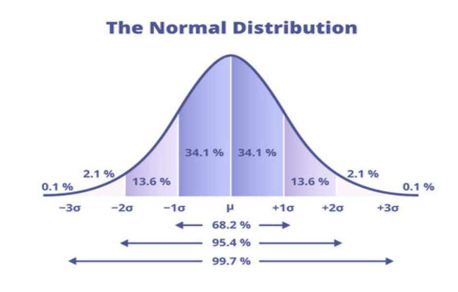
Normal Distibution Curve

Control Limits

The use of control limits allows someone to look at the variation of a product and make sure that it is within the expected limits. Typically, there are multiple samples analyzed for variation. But, even by just looking at where the values lie within the control limits, we can make some conclusions about what might have gone wrong when making the product in one sample. To find the control limits you must know the mean and standard deviation of your sample. The upper and lower control limits can be calculated using these equations

• UCL = x - (-L × s)
• LCL = x - (L × s)
• L is the number of standard deviations from the control mean you want to evaluate. The typical value used for L is 3.

Process Capability

Process capability analysis uses data from an initial sample to predict whether or not a manufacturing process will produce parts within certain specifications. When creating the process, the goal is to have all the products fall between an upper and lower specification limit. Process capability measures how consistently the products fall within the limits. An ideal process has its product parameters centered around a desired value and has a spread narrower than the specification width. To determine whether or not the process is ideal we need to calculate Cp and Cpk.

• Cp measures if the distribution can fit within the specification limit
  
  • Cp = USL-LSL / 6σ
• Cpk shows whether the average is centrally located within the specification limit
• Cpk = min(USL-𝛍 / 3σ , 𝛍-LSL / 3σ)
  *two equations, the minimum value of the equations is the Cpk